Results and (some) Discussion.
It was important to me to port the behavior of the calcBsImpVol.
An easy way to get the results visualized without using pytest and simialer
great tools is a unity plot.
The matrices/arrays which contain the values to be compared are flattened
to row vectors and scattered against each other. Any significant deviation will then
stand out from the line created by y = x
Couple of things which are left to point out in relation to Fig. 1, 2, 3 and 4:
Since I can’t know the assumptions made for the risk free rate and dividend yield I had to come up with somewhat reasonable assumptions on my own. As such, I picked the T-Notes yields corresponding with the options time until expiry as the risk free rate and the trailing 12m dividend payout as the dividend yield.
Fig 4.1, 4.2 and 4.3 illustrate that deviation is primarily an issue for calls.
bsimpv, calc_ivol and calcBsImpVol use closed form formulas designed to return the implied volatility of european options. The reference method however uses a numerical approach. american style options should generally be more expensive or equally priced to european style options.
A numerical approach seems to express that better for calls. Hence the implied volatility is underestimated by closed form approach.
About he puts with iVol ~ 0.5? Tell us.
reference vs calcBSImvol(), bsimpv() and calcbsimpvol()
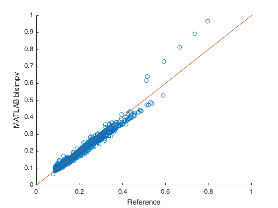
Fig. 1 - reference vs results of MATLAB builtin blsimpv()

Fig. 2 - reference vs results of MATLAB calcBSImpVol()
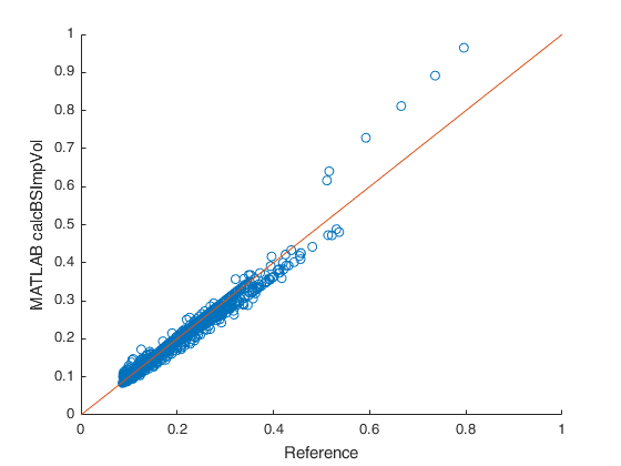
Fig. 3 - reference vs Python calcBSImpVol() - adjusted for NaN
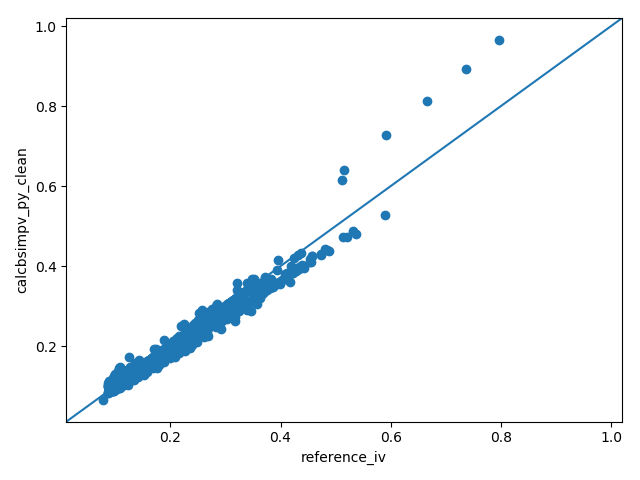
Fig. 4 - reference vs Python calcbsimpvol()

Fig. 4.1 - reference vs Python calcbsimpvol() - close up
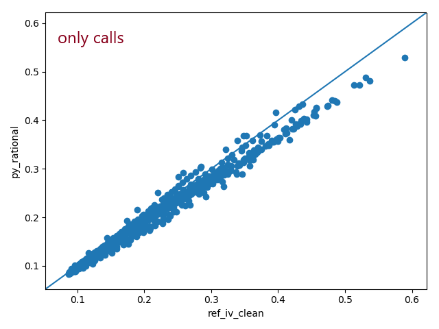
Fig. 4.2 - reference vs Python calcbsimpvol() - only calls
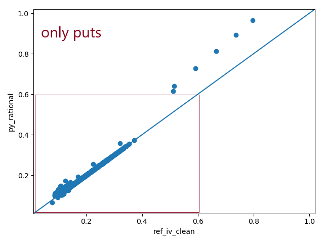
Fig. 4.3 - reference vs Python calc_ivol() - only puts
calcBSImvol vs bsimpv() vs calc_ivol
Fig. 5 shows that calcBSImvol() offers an extended calculation range compared to
bsimpv(). The NaN values returned from bsimpv() were set to zero in order to create Fig. 5.
Removing the “silent evindence” of ``NaN``s and ``zero``s returns Fig. 6.
Fig. 7 completes the picture.
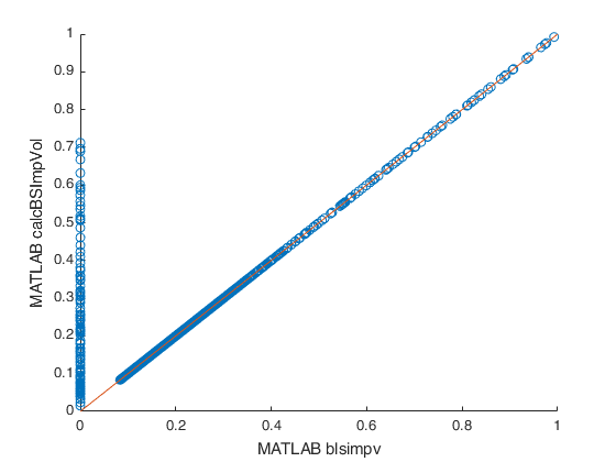
Fig. 5 - MATLAB builtin blsimpv() vs MATLAB calcBSImpVol()
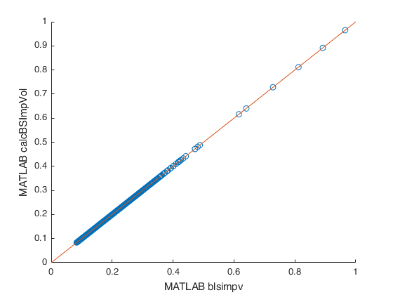
Fig. 6 - MATLAB builtin blsimpv() vs MATLAB calcBSImpVol() - adjusted for NaN
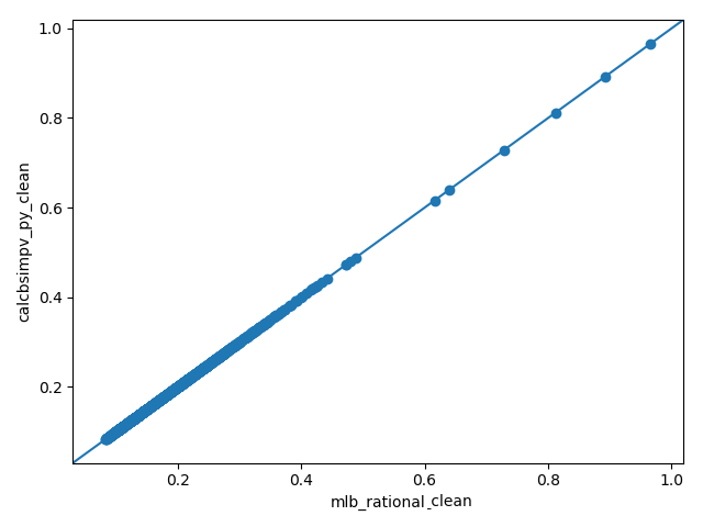
Fig. 7 - Python calcbsimpvol() vs MATLAB calcBSImVol()